Consider parts 1-2 as Agile for Data Scientists. This addendum could be considered Data Science for Agilists, and seeks to illustrate some of the fundamental concepts of data science and machine learning referred to in earlier posts.
Definitions: Data Science vs. Machine Learning
Data Science is a field that studies how to extract meaning from data, using a series of methods, algorithms, systems, and tools.
Machine Learning is a field devoted to understanding and building methods that utilize data to improve performance or inform predictions. Machine learning is considered a branch of artificial intelligence.
1. Learn patterns/relationships from existing data, and then to
2. Use those patterns to make predictions on new data
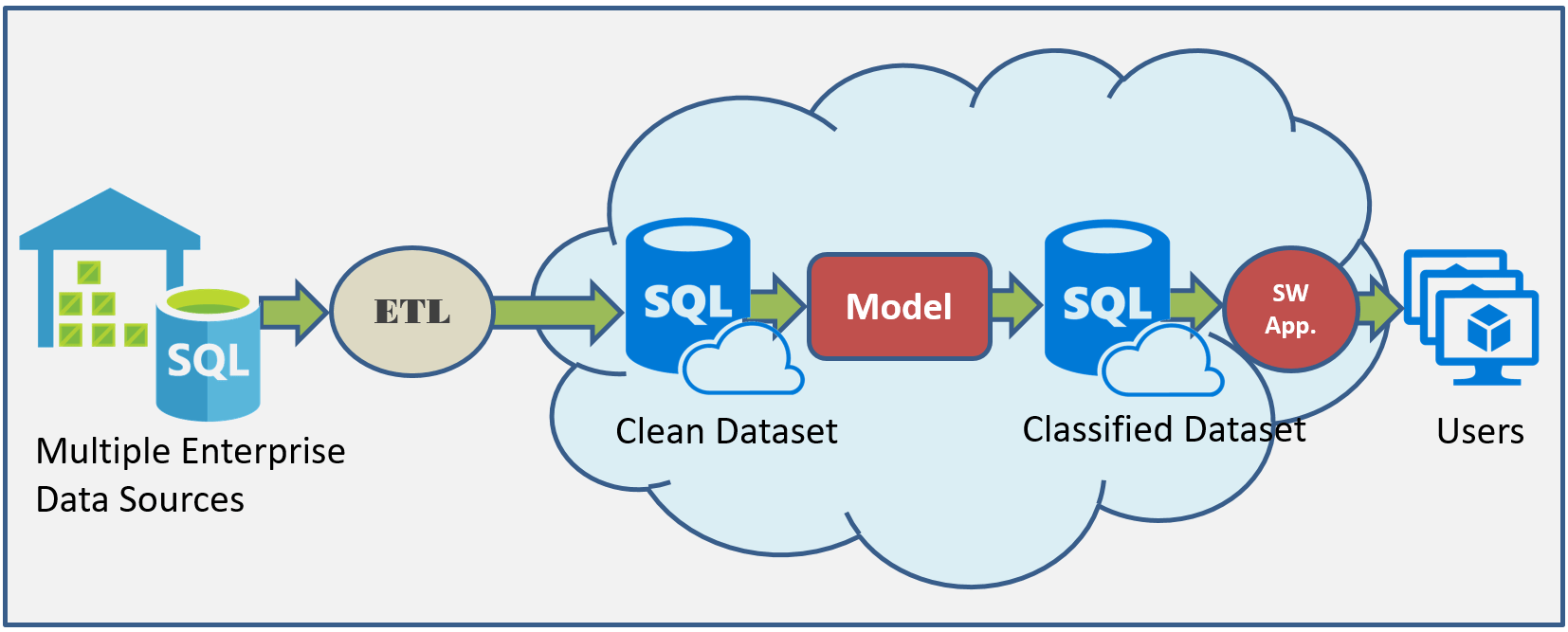
We’ll look at a fairly typical modeling project that uses a supervised learning approach. Supervised learning aims to produce models that can predict answers to questions like: which bank customers are most likely to default on a loan, or which cell phone service customers are most unlikely to renew their service contracts. Supervised means the models are trained on data that has been labelled with known outcomes for the question of interest. Models take in data that has been cleaned up and stripped down to its essential ‘features’ (predictor variables), and then use this data to make a prediction into which class (target variable) – e.g. renew/not renew – that the specific customer will belong to. The following diagram summarizes the key steps in this process.

Some models may simply predict a classification for a specific customer or sample instance – i.e. will renew/not renew their contracts, other models may go further and determine a probability or likelihood that the instance belongs to the class of interest.
Once we have constructed our model, it can be deployed and operationalized. In support of this we need processes and infrastructure in place to extract, clean, transform and consolidate data into a form that can be used by the model, and also software applications that can report model output to actual users.
Some Definitions:
- Features – (predictor variables) – training data input variables used to train a model. E.g. “age”, “income”, “loan amount.”
- Target – (target variables, or classes) – output from a trained model. E.g. “risk of default.”
- Training Data – a set of data used to train a model, comprising a set of input variables (features) and a known outcome (target).
- Test Data – a set of data used to test (or score) model performance after it has been trained.
Assuming we have a solid business problem statement with acceptance criteria or measurable success criteria (or a verifiable definition of MVP), then we would proceed along the following steps:
- Business Problem Definition: Microsoft, in their Team Data Science Process literature, talk about asking “sharp” questions that are relevant, specific and unambiguous, in order to clearly articulate the objectives of a data science project. Goals should be clear and have verifiable acceptance criteria, written in language understood by a business stakeholder (not a data scientist!). I have seen business epics for data science written like: Produce a model that performs with an AUC of 75%! Here’s a concise example from Eric Siegel’s book: Predictive Analytics – in a reference to a well publicized data science project at Target, where both the business problem/opportunity and intended application are defined:

- Data Identification: Identify the required data sources.
- Data Collection: Pull the initial data into the environment in which we run our analytics tools.
- Data Preparation: Removal of noise or errors in data, and identification of variables of interest. The data may then be consolidated into a single dataset, and loaded into an analytics environment where it can be processed by any required data mining tools – feature extraction, model generation, and so on. Prepared data can be separated into data used for training a model and data used for testing a model. Data preparation may be one of the most time-consuming parts of a data science project.
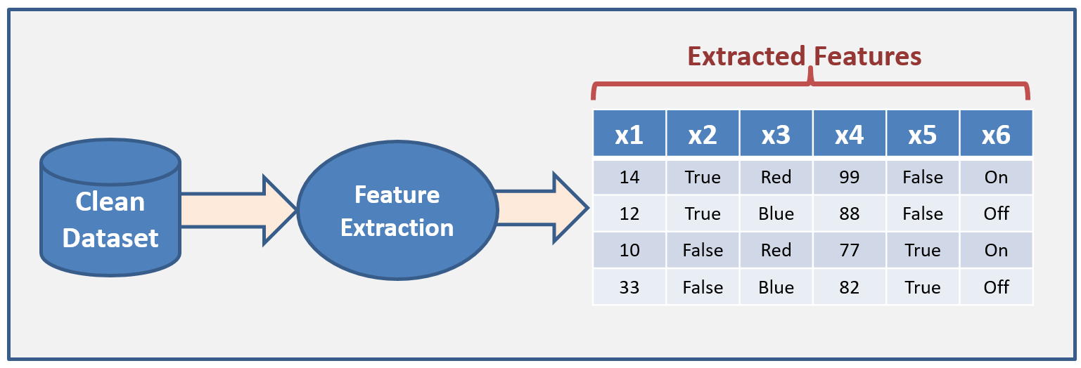
- Model Feature Extraction – Exploratory Data Analysis (EDA): The EDA step is to identify the variables that are the best discriminators for our desired classification (e.g. contract renew/not renew). EDA is usually performed using statistical techniques and tools like Pareto Analysis of the data – to determine quantitatively which variables have the biggest impact on the issue in question. This could be done with SQL queries and Group By clauses, however, there are many available tools to automate this process. The example in the diagram below shows a dataset with 6 features.
The resulting set of ‘features’, also known as predictor variables, may be refined by iteration in order to produce a model that meets the goal set out in the business definition. However, we can start with a simple model using a single predictor variable, say FICO Score, in our loan default example, (which we might believe is the single biggest driver of the loan default likelihood – we can arrive here via statistical analysis of the dataset), this would make our model a univariate model – that is, based on a single predictor variable. We would measure the performance of this model with one predictor and then add other predictor variables (income, age, marital status, …) assessing their impact on the accuracy of our predictions. This could be the basis of a strategy: build and deploy a simple univariate mode, then iterate with additional variables until the model performs to expectations.
- Model Development: Once we have our features selected, and have access to a labelled dataset – that is, a dataset for which the classification for each sample or record instance is known, we can run this training dataset through a learning algorithm (Naive Bayes, for example, for decision-tree type models) to generate the actual model. The result is that we now have a model that can potentially classify instances of new data. Again, there are many tools available to automate this process (we do not need to resort to coding thousands of lines of if-then-else statements).

- Model Testing: Models, having been trained on a labelled dataset may then be used to process new data and make predictions on how to classify each new record. Test the model using a test (unclassified) dataset and score its accuracy in classifying new data. Some subset, say 25%, of the original dataset is set aside for this purpose. There are various ways of measuring (or scoring) the model performance – Area Under ROC Curve – is one way. ROC AUC is a plot of the number of accurately classified records versus incorrectly classified records, where perfection = 1.0 (100%). So we can report things like: the model scores 75% for AUC.
- Model performance evaluation: Compare model performance (AUC score) versus previous iterations of the model, and against the goal defined in business problem statement/MVP. Continue to iterate on features and/or model parameters until a satisfactory performance is achieved.

- Model Deployment: If model meets MVP then deploy, else iterate to get more/better data.
Learn as Much as Possible (But not too Much)
Models can be modified iteratively and incrementally by exploring the decision-tree at progressively deeper levels. At some point we will run into diminishing returns, and may even overfit or overlearn with our model, which can result in model performance deterioration. The trick here is to be very clear about quantifying the original problem statement and getting into production with a model that delivers for the business.
References
- Predictive Analytics, Eric Siegel, Wiley, 2016
- Introduction to Pattern Recognition – very useful primer on basic data science concepts
- Microsoft Team Data Science Process
- Practical Data Science with Python